
This chapter follows the supplied KMU learning outcomes in a logical sequence. First understand what each statistical measure tells you, then practise choosing the correct measure for a given type of data, and finally revise the high-yield points at the end.
Descriptive Biostatistics and Data Distribution
Understand how a set of observations can be summarized by its typical value, spread and distribution, and how percentiles and the interquartile range help describe position within a dataset.
1. Topic Introduction
Descriptive biostatistics deals with methods used to organize, summarize and describe numerical data. A large collection of observations becomes easier to understand when we know its central or typical value, how widely the observations are spread around that value, and the shape of their distribution. Measures of central tendency such as the mean, median and mode describe the centre of a dataset, while measures of dispersion describe variability. The normal distribution provides an important model for understanding how many biological measurements are distributed. Percentiles and the interquartile range further show where an observation lies relative to the rest of the data. These concepts form the basis for interpreting medical and public-health data correctly.
A. Measures of Central Tendency: Core Idea and Classification
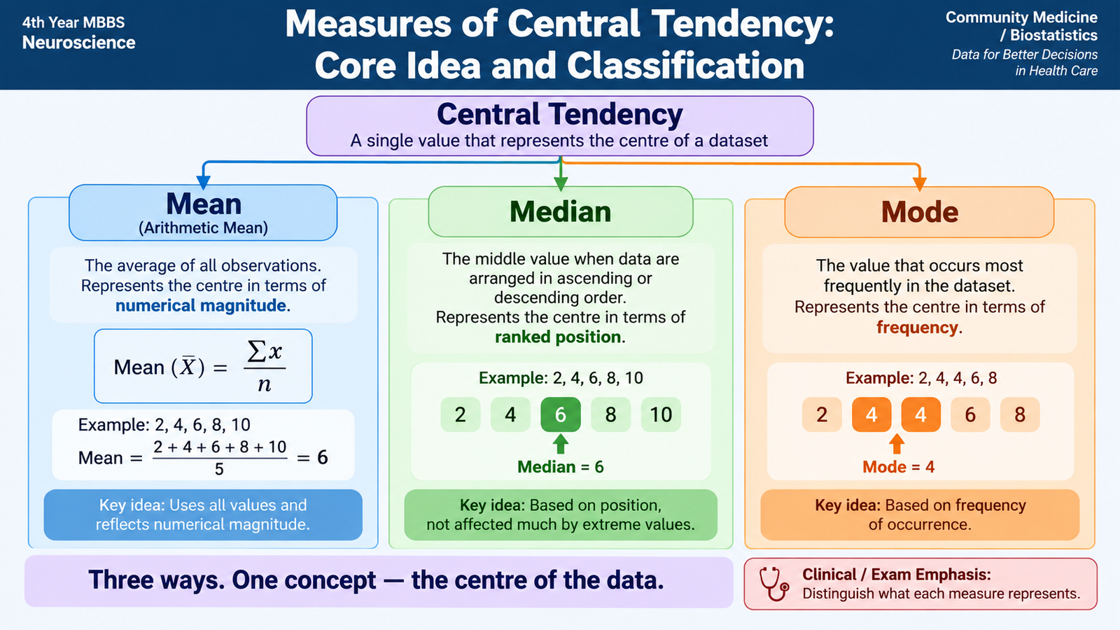
A dataset often contains many individual observations. Looking at every value separately may make it difficult to appreciate the overall pattern. A measure of central tendency summarizes the dataset using a value that represents its centre or typical level.
The three principal measures are mean, median and mode. They do not always give the same answer because each defines the “centre” in a different way.
Main measures
- Arithmetic mean: the sum of all observations divided by the number of observations.
- Median: the middle observation after the data have been arranged in ascending or descending order.
- Mode: the value that occurs most frequently.
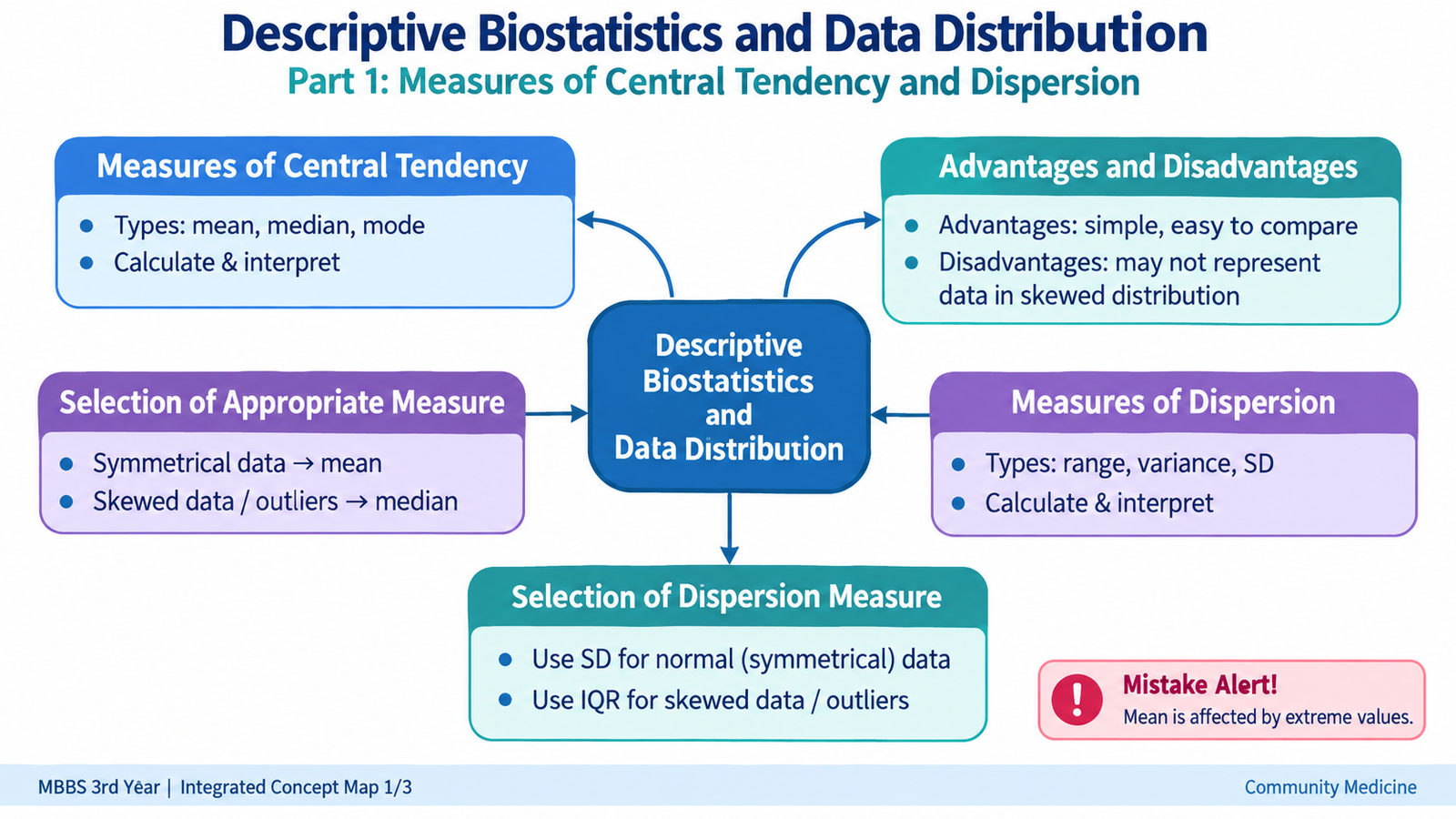
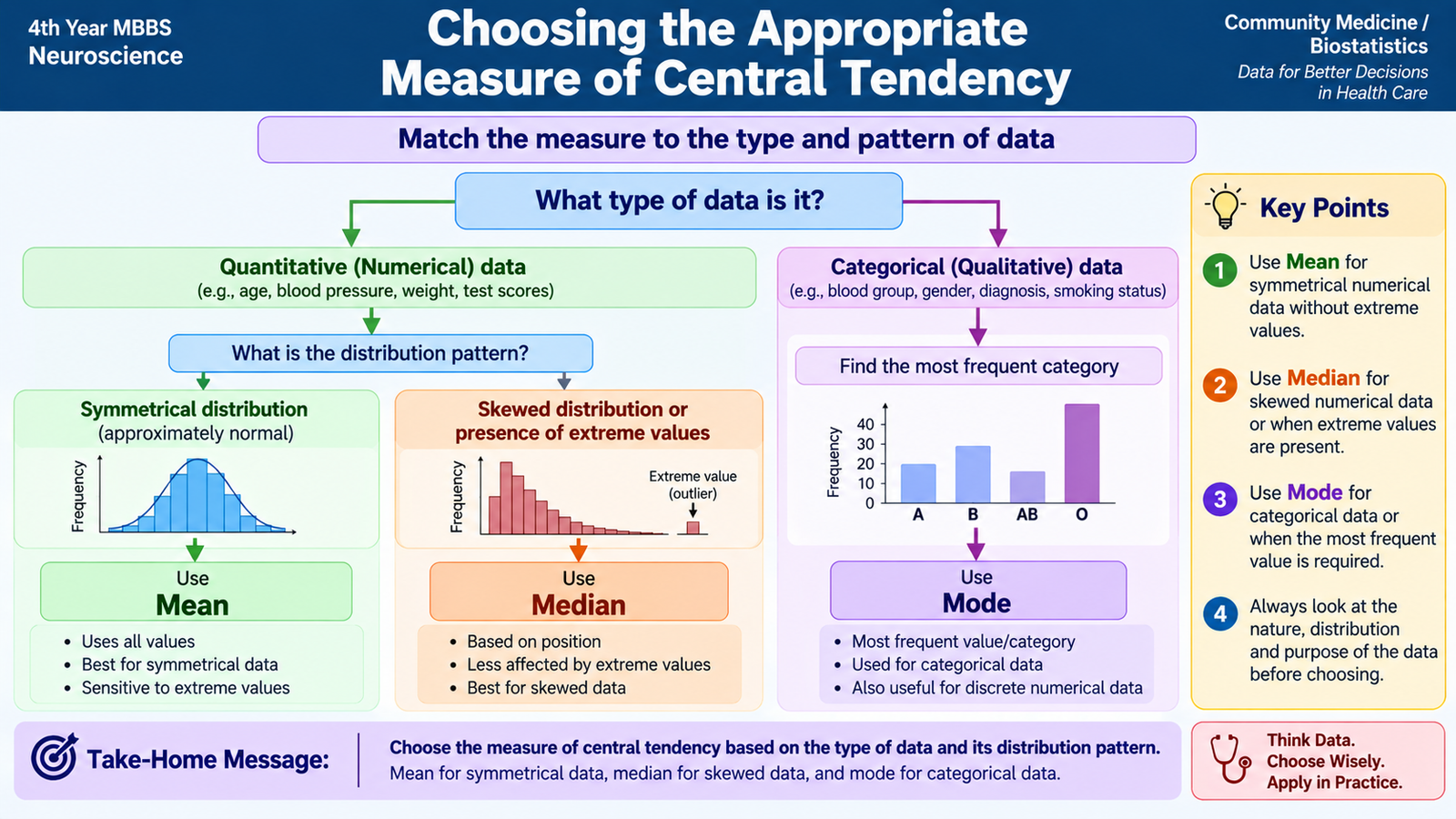
The choice between these measures depends mainly on the type of data and the shape of its distribution. The mean uses every numerical observation and is therefore highly informative, but it is also affected by extreme values. The median depends on position rather than magnitude, so it is more resistant to extreme observations. The mode identifies the most frequent category or value and can therefore be used even for categorical data.
B. Calculating and Interpreting Mean, Median and Mode
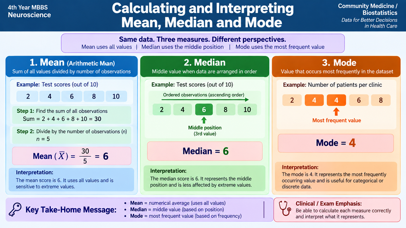
Knowing the definition of a measure is not enough. A student should also understand how it is calculated and what the resulting number actually means. Consider the following simple dataset representing five observations:
Arithmetic mean
The arithmetic mean uses the numerical value of every observation.
Mean = (4 + 5 + 6 + 7 + 8) ÷ 5 = 6
A mean of 6 means that 6 represents the mathematical centre of these observations. The individual observations do not need to equal 6; it is a summary of the complete dataset.
If frequencies are given, each value contributes according to how frequently it occurs:
where x is the observed value and f is its frequency.
Median
To calculate the median, first arrange the observations in order. If the number of observations is odd, the median is the single middle observation.
Therefore, the median = 6.
If there is an even number of observations, there are two middle values. Their arithmetic mean is taken as the median.
Median = (4 + 6) ÷ 2 = 5.
The median divides an ordered dataset into two halves: approximately half the observations lie below it and half lie above it.
Mode
The mode is found by identifying the value occurring most often.
A dataset may have one mode, more than one mode, or no clear mode when no value occurs more frequently than the others.
C. Choosing the Appropriate Measure of Central Tendency
No single measure of central tendency is best for every dataset. The correct choice depends on whether the data are numerical or categorical, whether the numerical distribution is symmetrical or skewed, and whether extreme observations are present.
The mean is generally most informative for quantitative data with a reasonably symmetrical distribution because every observation contributes to it. However, this same property makes it sensitive to very high or very low values.
The median is especially useful when a distribution is skewed. Because it depends mainly on the ranked position of observations, an extreme value has much less effect on it. The mode is useful when the most commonly occurring value or category is important and is the only one of the three that can naturally summarize purely nominal categories.
Effect of an extreme value
Consider the observations:
The unusually high value of 30 pulls the mean upward, whereas the median remains the middle value, 4. This explains why the median often represents the centre of a markedly skewed distribution more realistically.
Important comparison
| Feature | Mean | Median | Mode |
|---|---|---|---|
| Basis | Magnitude of all observations | Ranked position | Frequency |
| Effect of extremes | Markedly affected | Little affected | Usually little affected |
| Best suited to | Symmetrical quantitative data | Skewed quantitative or ordered data | Most frequent value or category |
| Main advantage | Uses all observations | Resistant to extremes | Simple and usable for categories |
| Main disadvantage | Distorted by outliers and skewness | Does not use the magnitude of every observation | May be absent or multiple |
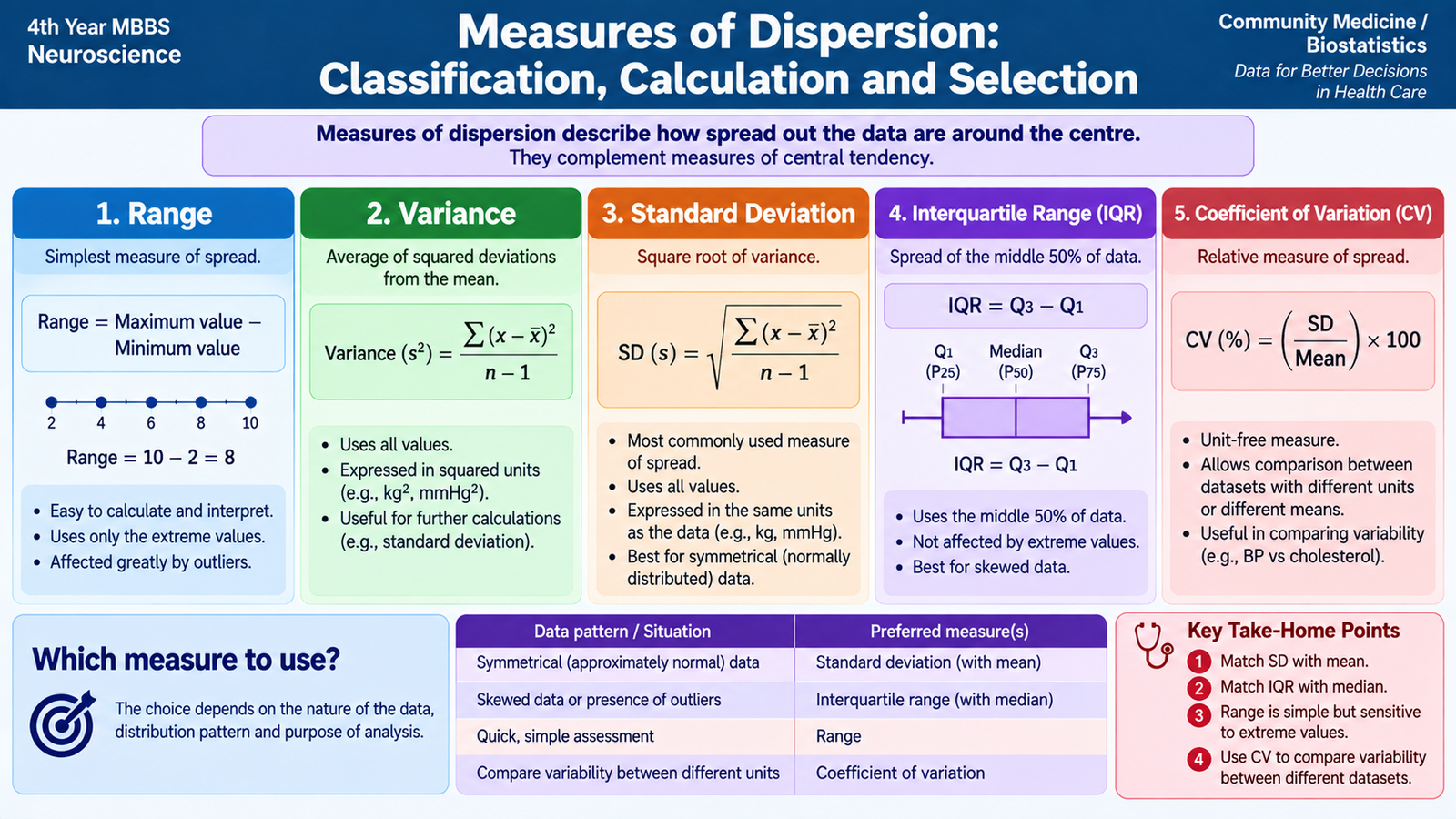
D. Measures of Dispersion: Classification, Calculation and Selection
Two datasets may have the same mean but still be very different. One may have values closely clustered around the centre, while another may contain values spread over a wide range. Dispersion describes this variability or spread.
Measures of dispersion are therefore interpreted together with a measure of central tendency. The centre tells us where the data are located; dispersion tells us how closely the observations are grouped around that centre.
Classification
Measures may be expressed in the original units of measurement or as relative measures that allow comparison between datasets.
- Absolute measures: range, interquartile range, quartile deviation, mean deviation, variance and standard deviation.
- Relative measure: coefficient of variation.
1. Range
The range is the simplest measure of dispersion.
For the observations 4, 5, 6, 7 and 8, the range is 8 − 4 = 4.
Its main advantage is simplicity. Its major limitation is that it depends only on the two extreme observations and ignores all values between them.
2. Mean deviation
Mean deviation is based on the average of the absolute differences between individual observations and a central value. It therefore uses more information than the range. Absolute differences are used so that positive and negative deviations do not cancel each other.
3. Variance
Variance measures the average squared deviation of observations from their mean. Squaring prevents positive and negative deviations from cancelling and gives greater weight to observations that lie farther from the mean.
Because variance is expressed in squared units, it is mathematically useful but less intuitive for direct clinical interpretation.
4. Standard deviation
The standard deviation (SD) is the square root of the variance. It is one of the most commonly used measures of dispersion because it uses all observations and is expressed in the same units as the original measurement.
A small SD means that observations are relatively close to their mean. A large SD indicates greater spread.
5. Interquartile range
The interquartile range describes the spread of the middle half of the observations:
Because the lowest and highest quarters are excluded, the IQR is much less influenced by extreme values than the range or standard deviation. It is therefore particularly useful for skewed data.
6. Coefficient of variation
The coefficient of variation expresses the standard deviation relative to the mean and is commonly presented as a percentage:
Because it is relative rather than expressed in the original measurement units, it is useful when comparing variability between datasets whose means or measurement scales differ appropriately.
Selecting the appropriate measure of dispersion
| Situation | Useful measure | Reason |
|---|---|---|
| Quick description of total spread | Range | Simple maximum-to-minimum spread |
| Symmetrical quantitative data summarized by mean | Standard deviation | Uses all observations and describes spread around mean |
| Skewed data or important outliers | Interquartile range | Resistant to extreme observations |
| Comparison of relative variability | Coefficient of variation | Expresses spread relative to the mean |
E. Normal Distribution: Definition, Graph and Significance
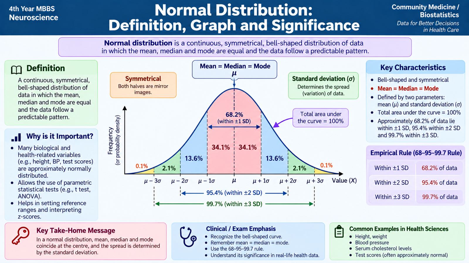
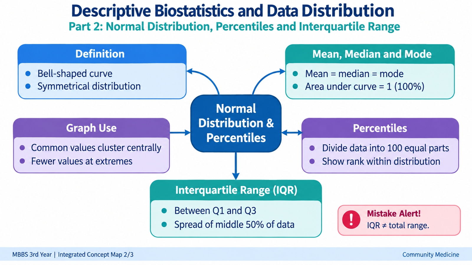
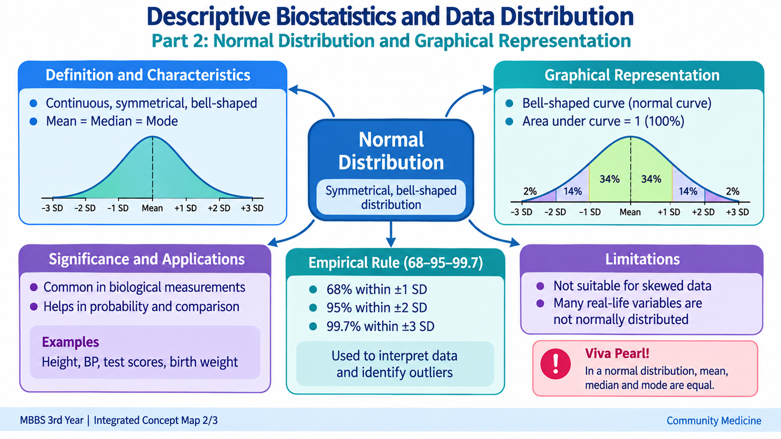
A normal distribution is a continuous, symmetrical, bell-shaped distribution in which observations are concentrated around a central value and become progressively less frequent toward either extreme.
The normal distribution is important in biostatistics because many biological measurements approximate this pattern. It also provides a useful framework for understanding how observations relate to the mean and standard deviation.
Characteristics of the normal distribution
- It is symmetrical around its centre.
- It has a single peak and is therefore unimodal.
- The mean, median and mode coincide at the centre.
- The curve falls smoothly on both sides of the centre.
- The tails approach the horizontal axis but do not abruptly end.
- The total area under the curve represents the whole distribution.
- The mean determines the central location of the curve.
- The standard deviation determines how narrow or widely spread the curve is.
Relationship with standard deviation
In an ideal normal distribution, observations occur in a predictable pattern around the mean:
- Approximately 68% lie within one standard deviation on either side of the mean.
- Approximately 95% lie within two standard deviations.
- Approximately 99.7% lie within three standard deviations.
This pattern explains why standard deviation is especially meaningful when quantitative observations are approximately normally distributed.
Graphical representation
When frequency is plotted against increasing values of a normally distributed variable, the graph forms the characteristic bell-shaped curve. The highest point occurs around the mean. Equal horizontal distances to the left and right of the mean correspond to equal numbers of standard deviations.
A narrow curve indicates less variability and therefore a smaller SD. A broader, flatter normal curve indicates greater variability and a larger SD. The mean may remain the same even though the spread differs.
Significance
Recognizing normality helps determine how data should be summarized. Approximately symmetrical normally distributed data are usually described using the mean together with the standard deviation. If the distribution is markedly skewed, the median and interquartile range often provide a more representative description.
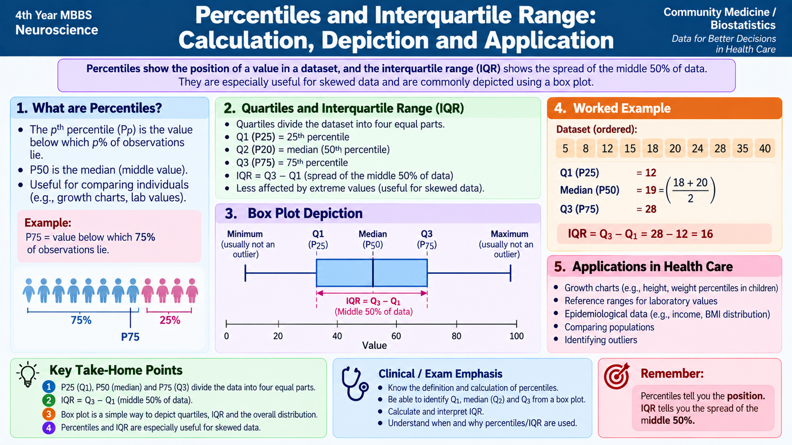
F. Percentiles and Interquartile Range: Calculation, Depiction and Application
A percentile describes the position of an observation relative to an ordered dataset. The kth percentile is the value below which approximately k percent of the observations lie. Percentiles therefore describe relative position rather than simply the centre or overall spread.
For example, the 50th percentile represents the middle position of an ordered distribution and corresponds to the median.
Relationship between percentiles and quartiles
- Q1: first quartile = 25th percentile.
- Q2: second quartile = 50th percentile = median.
- Q3: third quartile = 75th percentile.
The first and third quartiles enclose the central half of the observations. The distance between them is the interquartile range.
Calculating a percentile in ungrouped data
The observations are first arranged in ascending order. A commonly used rank approach locates the required percentile using:
where k is the required percentile and n is the number of observations. When the calculated position lies between two observations, interpolation may be used. Slightly different rank conventions may be used in different statistical systems, but the underlying idea remains the same: ordered observations are divided according to cumulative position.
Simple IQR example
Consider an ordered set in which Q1 has been identified as 12 and Q3 as 20.
IQR = 20 − 12
IQR = 8
This means that the middle 50% of observations occupy a span of 8 units.
Graphical depiction
Percentiles can be identified from an ordered cumulative distribution. On a cumulative frequency curve, the required cumulative percentage can be located and projected to the measurement axis to estimate the corresponding percentile.
Quartiles and the IQR are also represented clearly by a box-and-whisker plot. The lower edge of the box corresponds to Q1, the line inside the box represents the median, and the upper edge represents Q3. The length of the box therefore represents the IQR.
Applications
Percentiles are particularly useful when the relative position of an individual observation is more meaningful than its absolute numerical value. They can show whether an observation lies relatively low, around the middle, or relatively high within a reference distribution.
The IQR is especially useful for skewed data because it summarizes the spread of the middle half of observations without being strongly influenced by very low or very high extreme values. For this reason, the median and IQR are commonly interpreted together.
⭐ AIM High-Yield Review
🎥 Video Learning — Descriptive Biostatistics & Data Distribution
Review measures of central tendency, measures of dispersion, percentiles, interquartile range and the normal distribution.