
This chapter follows the KMU learning outcomes and builds inferential biostatistics in a logical sequence. First understand what each statistical idea means and why a test is selected; then use the final high-yield review for revision.
Inferential Biostatistics: Confidence Intervals, Hypothesis Testing and Statistical Tests
Understand how a sample is used to make conclusions about a population, how uncertainty is measured, how hypotheses are tested, and how Z, t, chi-square, correlation and regression are selected and interpreted.
1. Topic Introduction
Inferential biostatistics allows a researcher to use information obtained from a sample to make a reasoned conclusion about the larger population from which that sample came. Because different samples give slightly different results, every estimate contains some uncertainty. This uncertainty can be described using the standard error and confidence interval. Hypothesis testing then helps determine whether an observed difference or association is reasonably compatible with chance alone. In this chapter, you will learn confidence intervals, P values, statistical errors, distribution shapes, selection of parametric and non-parametric tests, and the calculation and interpretation of Z, t and chi-square tests. You will also learn correlation, regression and common practical problems encountered when using statistical methods and SPSS.
A. Standard Error, Confidence Level and Confidence Interval
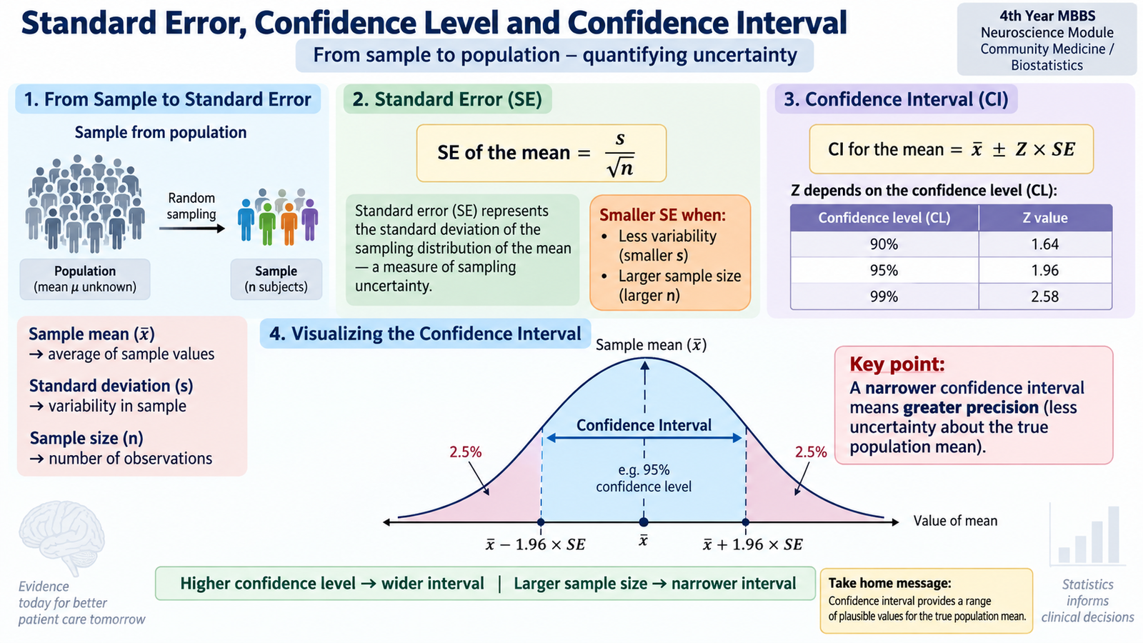
A sample statistic, such as a sample mean, is an estimate of the true population value. If several samples are taken from the same population, their means will not be exactly identical. This natural sample-to-sample variation is called sampling variation. Inferential statistics measures this uncertainty rather than pretending that the sample estimate is exact.
Standard error
The standard error (SE) describes how much a sample statistic is expected to vary from one sample to another. For a sample mean:
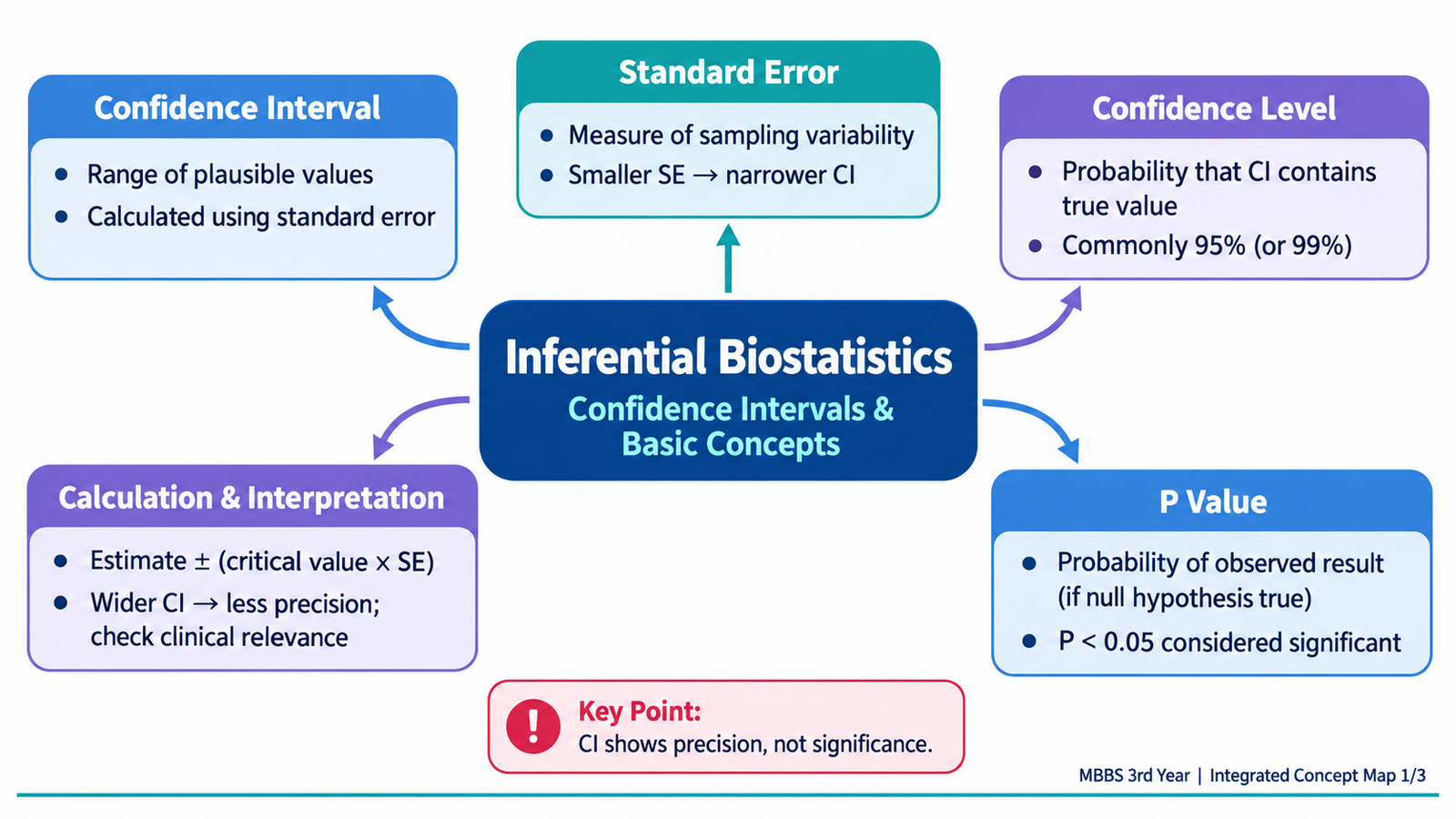
Here, SD describes variation among individual observations, whereas SE describes the precision of the estimated sample mean. Increasing the sample size increases the denominator √n and therefore reduces the SE. A smaller SE means a more precise estimate.
Confidence level
The confidence level describes the long-run reliability of the method used to construct a confidence interval. A commonly used confidence level is 95%. Higher confidence requires a wider interval because we demand greater assurance that the procedure captures the true population value.
Confidence interval
A confidence interval (CI) gives a range of plausible values for the unknown population parameter. Its general form is:
For a large-sample estimate using the normal approximation, a 95% CI is commonly calculated as:
Example: If a sample mean is 120 and its SE is 2, the approximate 95% CI is 120 ± (1.96 × 2), giving about 116.1 to 123.9.
The correct interpretation is that if the sampling process were repeated many times and an interval were constructed in the same way each time, approximately 95% of those intervals would contain the true population parameter. Once one particular interval has been calculated, the true parameter is fixed; therefore, it is better not to say that there is a “95% probability” that the fixed parameter lies inside that particular interval.
B. Hypothesis Testing, P Value and Statistical Errors
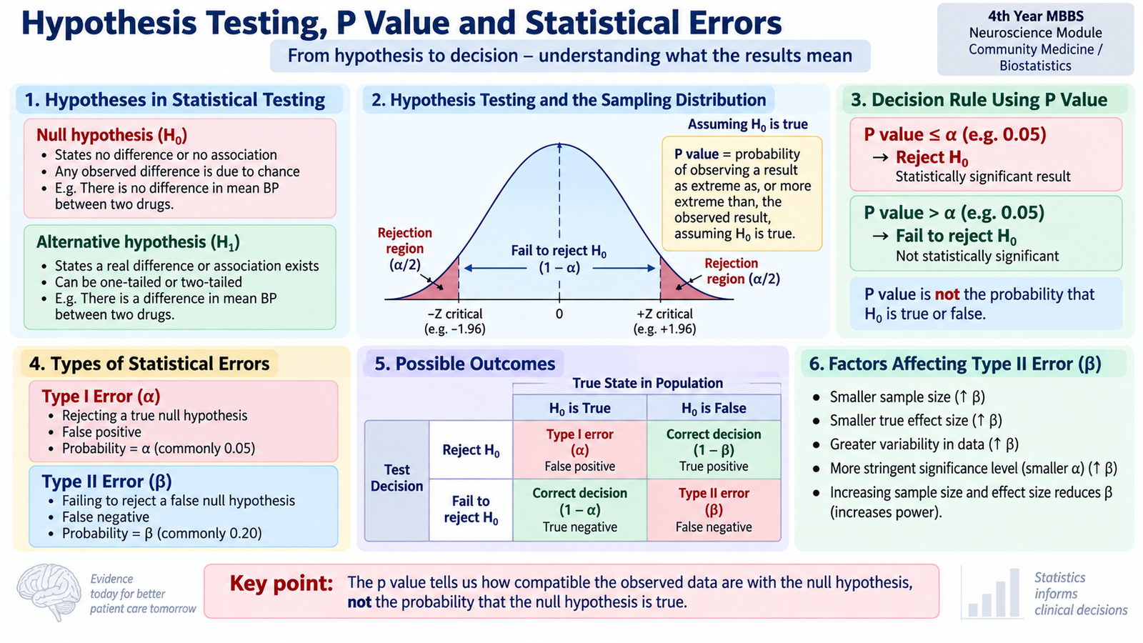
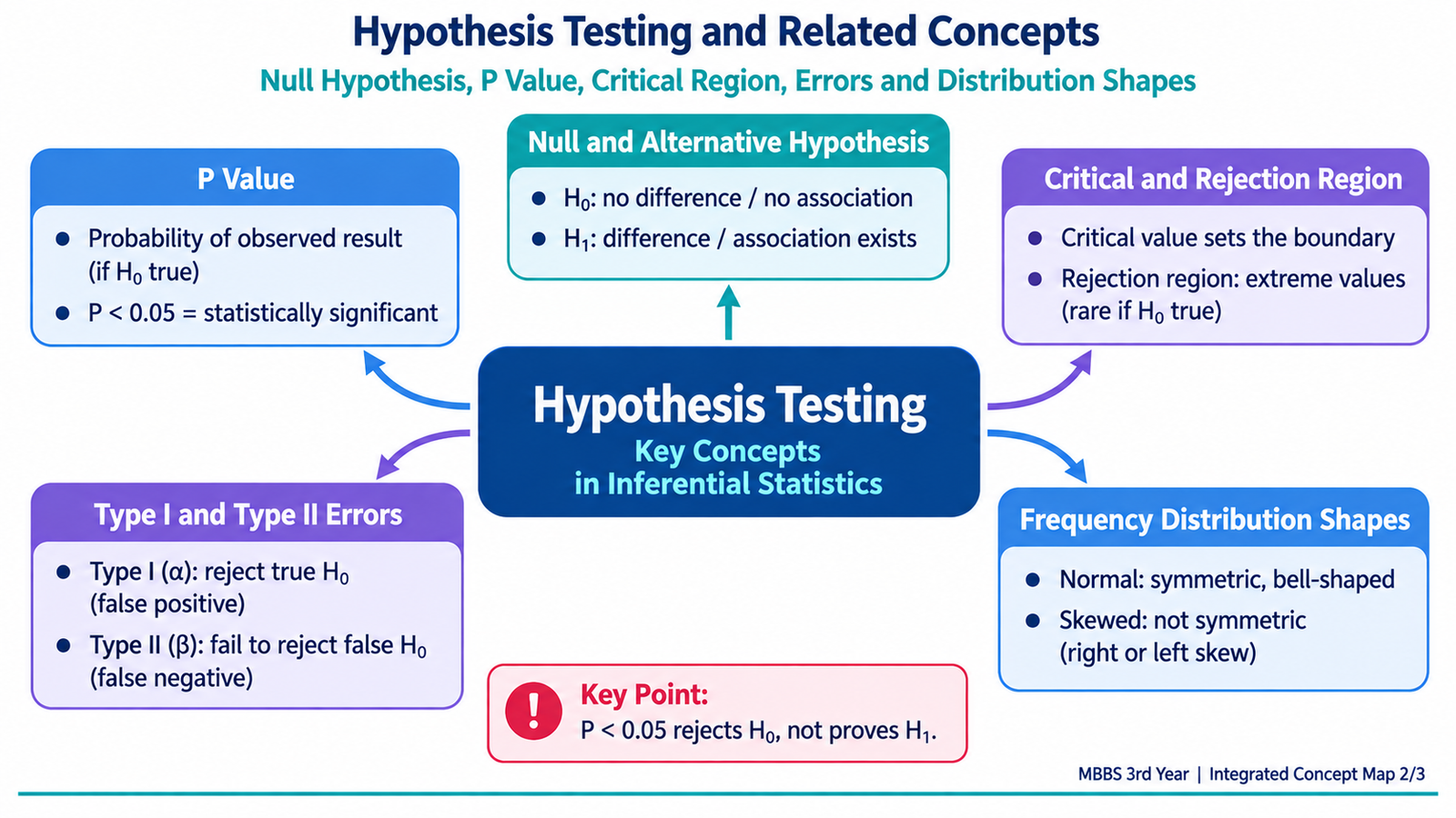
Hypothesis testing provides a structured way to decide whether an observed sample result is sufficiently unusual to provide evidence against a stated assumption. The starting assumption is the null hypothesis (H0). It usually states that there is no difference, no association or no effect. The alternative hypothesis (H1) states that a difference, association or effect exists.
P value
The P value is the probability, assuming the null hypothesis is true, of obtaining the observed result or a result more extreme than the one observed. A small P value means that the data would be unusual if H0 were true.
The researcher selects a significance level, α (alpha), before interpreting the test. If P is less than the selected α level, H0 is rejected. If P is not less than α, there is insufficient evidence to reject H0.
Critical and rejection regions
A statistical test has a sampling distribution expected under H0. The critical value marks the boundary beyond which a result is considered sufficiently unlikely under H0. Values beyond this boundary form the rejection region or critical region.
For a two-sided test, rejection regions are placed in both tails because sufficiently large differences in either direction may contradict H0. The selected α level determines how much of the distribution is assigned to the rejection region.
Alpha and beta errors
No statistical decision is completely free from the possibility of error.
- Type I error (α): rejecting H0 when H0 is actually true. This is a false-positive statistical conclusion.
- Type II error (β): failing to reject H0 when an important real difference or association actually exists. This is a false-negative statistical conclusion.
- Statistical power = 1 − β: the ability of a study to detect a real effect when it exists.
Power generally improves when the sample size is larger, the true effect is larger, or random variability is lower. Therefore, failure to obtain statistical significance does not necessarily prove that two groups are identical.
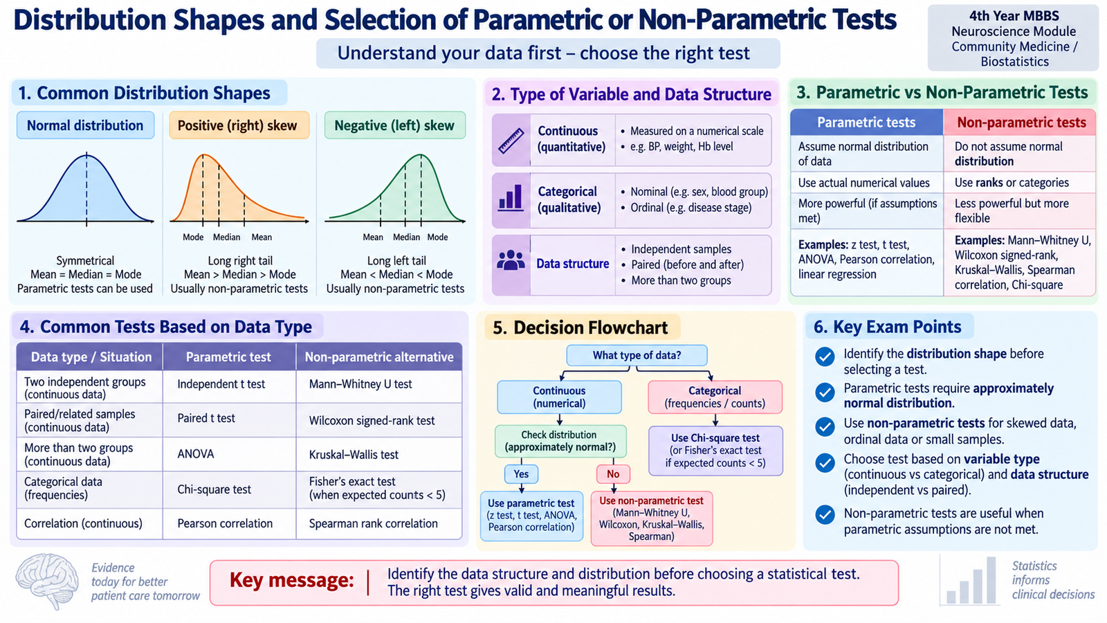
C. Distribution Shapes and Selection of Parametric or Non-Parametric Tests
Before selecting a statistical test, the researcher must understand the type and distribution of the data. A statistical test that is suitable for normally distributed continuous measurements may be inappropriate for markedly skewed data, ranks or categorical observations.
Frequency-distribution shapes
A frequency distribution shows how observations are spread across different values. The shape of the distribution affects how the data should be summarized and which statistical methods are appropriate.
- Normal distribution: symmetrical and bell-shaped. Mean, median and mode lie approximately at the centre.
- Positively skewed distribution: has a longer tail toward higher values. A few very high observations pull the mean upward.
- Negatively skewed distribution: has a longer tail toward lower values. A few very low observations pull the mean downward.
- Other irregular shapes: distributions may contain several peaks, gaps or extreme observations. Such findings should be examined rather than ignored.
Parametric tests
Parametric tests make assumptions about the distribution and characteristics of the population from which the data are sampled. They are mainly used with numerical measurements when their assumptions are reasonably satisfied. They usually make fuller use of the numerical information and can be statistically efficient when appropriately applied.
Non-parametric tests
Non-parametric tests require fewer assumptions about the underlying distribution. They are useful for ordinal or ranked information and may also be appropriate for numerical data that do not satisfy the assumptions of a suitable parametric test.
Selection should not be based on one rule alone. The investigator should consider the research question, variable type, number of groups, whether observations are independent or paired, and the shape and assumptions of the data.
D. Z Test
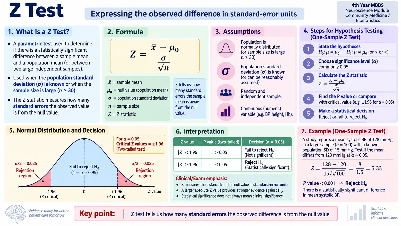
The Z test uses the standard normal distribution to determine how far an observed sample result lies from the value expected under the null hypothesis. It is particularly useful when the sampling distribution can reasonably be treated as normal, such as in sufficiently large samples, and in situations where the relevant population variability is known. Z procedures are also commonly used for proportions when normal-approximation conditions are satisfied.
Basic calculation for one mean
Here, x̄ is the observed sample mean, μ0 is the population mean stated by H0, σ is the population standard deviation, and σ/√n is the standard error.
The numerator measures the observed difference from the null value. Dividing by the standard error expresses that difference in standard-error units. Therefore, the farther the Z value lies from zero, the less compatible the observation is with H0.
Application in hypothesis testing
- State H0 and H1.
- Select the significance level.
- Calculate the standard error.
- Calculate Z.
- Compare the result with the appropriate critical region or obtain its P value.
- Reject or fail to reject H0 and interpret the result in the context of the research question.
Example of interpretation: Suppose a researcher asks whether the mean systolic blood pressure in a large sample differs from a specified population value. A Z statistic far into the rejection region would provide evidence against the stated null value, whereas a Z value near zero would indicate that the observed difference is small relative to its sampling uncertainty.
E. t Test and Degrees of Freedom
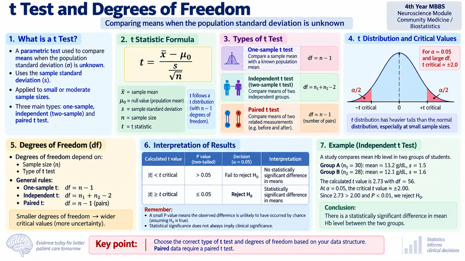
The t test is used to compare means when the population standard deviation is not known and must be estimated from the sample. Because this introduces additional uncertainty, the test uses the t distribution rather than the standard normal distribution. The t distribution has wider tails, especially when the sample is small. As the sample size and degrees of freedom increase, it increasingly resembles the normal distribution.
Common forms of the t test
- One-sample t test: compares one sample mean with a specified reference mean.
- Independent-samples t test: compares the means of two independent groups.
- Paired t test: compares two related measurements, such as measurements taken before and after an intervention in the same individuals.
One-sample calculation
The structure resembles the Z statistic, but the sample standard deviation s is used to estimate population variability.
Degrees of freedom
Degrees of freedom (df) describe how much independent information is available for estimating variability. For a one-sample t test, df = n − 1. The paired t test also uses n − 1, where n is the number of pairs. For the conventional equal-variance independent-samples t test, df = n1 + n2 − 2.
Degrees of freedom matter because the critical t value depends on them. With fewer degrees of freedom, greater uncertainty produces wider tails and a more extreme t value is required for the same significance level.
Hypothesis testing and interpretation
The calculated t value is assessed using its t distribution and degrees of freedom. The resulting P value is then interpreted against the preselected α level. A statistically significant result indicates evidence of a difference in means; it does not by itself establish that the difference is clinically important.
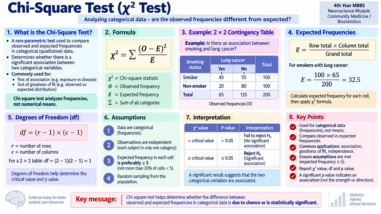
F. Chi-Square Test
The chi-square (χ²) test is mainly used with categorical data expressed as frequencies or counts. Instead of comparing numerical means, it compares the number of observations actually seen with the numbers that would be expected if the null hypothesis were true.
Main uses
- Test of association or independence: determines whether two categorical variables are associated.
- Goodness-of-fit test: determines whether observed frequencies follow a specified expected distribution.
Calculation
O represents the observed frequency and E the expected frequency. If observed and expected frequencies are very similar, χ² will be small. Larger discrepancies produce a larger χ² value and provide stronger evidence against H0.
For a contingency table, the expected frequency of an individual cell is calculated as:
Degrees of freedom
Hypothesis testing and interpretation
For a test of association, H0 states that the categorical variables are independent. The calculated χ² value and its degrees of freedom are used to obtain a P value. A sufficiently small P value supports rejection of independence and suggests statistical evidence of an association.
The test requires independent observations and relies on expected frequencies being sufficiently adequate for the chi-square approximation. Very small expected cell frequencies can make the approximation unreliable and may require an exact statistical approach instead.
G. Correlation, Regression and Practical Application in SPSS
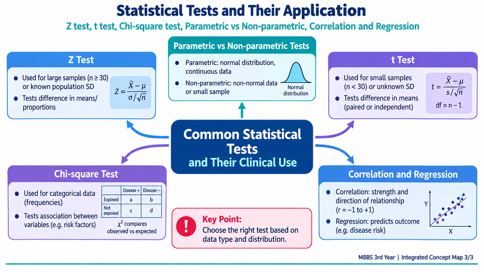
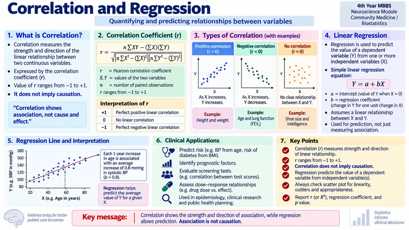
Correlation and regression both examine relationships between variables, but they answer different questions. Correlation describes the direction and strength of an association. Regression goes further by describing how an outcome changes in relation to one or more explanatory variables and can be used for prediction.
Correlation
A correlation coefficient summarizes the degree to which two variables vary together. For a linear relationship between suitable continuous variables, the Pearson correlation coefficient r ranges from −1 to +1.
- r near +1: strong positive linear relationship.
- r near −1: strong negative linear relationship.
- r near 0: little or no linear relationship.
A positive correlation means that higher values of one variable tend to occur with higher values of another. A negative correlation means that higher values of one tend to occur with lower values of the other.
When variables are ranked or when the assumptions for Pearson correlation are not suitable, a rank-based correlation method such as Spearman correlation may be more appropriate.
Regression
Simple linear regression models the relationship between a continuous outcome Y and an explanatory variable X:
a is the intercept and b is the regression coefficient or slope. The slope estimates the expected change in Y associated with a one-unit change in X.
For example, regression may be used to describe how systolic blood pressure changes with age or how a laboratory measurement changes in relation to another continuous predictor. The regression equation can also be used to estimate expected values, provided prediction remains appropriate for the population and range of data studied.
Practical and conceptual problems in biostatistics and SPSS
Statistical software performs calculations quickly, but it does not decide whether the analysis is scientifically appropriate. Most errors occur before or after the computer produces the result.
- Wrong variable definition: numerical, ordinal and categorical variables require different analyses.
- Incorrect data coding: inconsistent codes can produce misleading tables and analyses.
- Missing data: missing observations must be recognized rather than accidentally treated as genuine values.
- Outliers: unusual observations can strongly influence means, correlation and regression.
- Ignoring distribution and assumptions: selecting a test only because it is familiar can produce invalid conclusions.
- Independent versus paired data: confusing these structures may lead to selection of the wrong test.
- Reading only the P value: interpretation should also consider the effect estimate, confidence interval and clinical meaning.
- Statistical versus clinical significance: a very small difference may become statistically significant in a large sample yet remain clinically unimportant.
A practical SPSS reasoning sequence
3. Integrated Mechanism Flow
Inferential analysis can be understood as one connected decision pathway:
Define what is being estimated or tested.
State the statistical hypotheses.
Identify variable type, pairing and distribution.
Choose Z, t, chi-square or another suitable method.
Obtain test statistic, SE, CI and/or P value.
Compare P with α or assess the critical region.
Combine statistical evidence with precision and clinical meaning.
4. Important Comparison
Parametric versus Non-Parametric Tests
| Feature | Parametric Tests | Non-Parametric Tests |
|---|---|---|
| Main data | Usually numerical measurements | Often ordinal, ranks or unsuitable non-normal numerical data |
| Distribution assumptions | Greater distributional assumptions | Fewer distributional assumptions |
| Typical examples | Z test, t test, Pearson correlation | Rank-based tests, Spearman correlation; chi-square is used for categorical frequencies |
| Selection | Use when relevant assumptions are reasonably satisfied | Useful when data structure or assumptions do not suit the corresponding parametric method |
Choosing Among Common Tests
| Method | Main Question | Main Data | Key Point |
|---|---|---|---|
| Z test | Does an estimate differ from the null value? | Means or proportions under suitable normal-approximation conditions | Uses standard normal distribution |
| t test | Do one or two means differ? | Continuous numerical data | Uses estimated SD and degrees of freedom |
| Chi-square | Are categorical frequencies associated or different from expectation? | Counts/frequencies | Compares observed with expected frequencies |
| Correlation | How strongly do two variables move together? | Paired measurements or ranks | Association does not prove causation |
| Regression | How does an outcome change with an explanatory variable? | Outcome and predictor variables | Provides an equation and estimated slope |
⭐ AIM High-Yield Review
🎥 Video Learning — Inferential Biostatistics
Review the selection and interpretation of Z test, t test, chi-square test, correlation and regression.